Data transformations, normalization, standardization
Missing values imputation
Dummy variables
Data visualization (2D and 3D)
Descriptive analytics-case study covering data manipulation, measures of central tendency, measures of dispersion, measures of distribution, measures of associations, t-test, Hypothesis testing (t-test, ANOVA, Chi Squared Test, F-Test), basic statistical modeling framework
To start with content of this chapter, we need to create a new project. Let’s create new project with this sequence:
-> Go to File tab -> Click New Project tab -> In New Project Wizard, click New Project Directory -> In New Project Wizard, click Project Type: Quarto Project
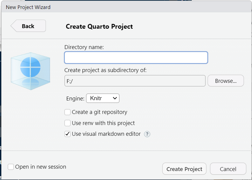
Now you see, following window:
In this window, give name to your directory in the box “Directory Name” and set the directory path with browse option. Now, click the Create Project tab to start your first ever project. This is how your workspace will look like:
In the output pane (in blue circle), you can see that there are three files are created- _quarto.yml, name.qmd and name.Rproj. Here “name” is inherited from directory name we have given while setting the project. You can give any name by selecting the .qmd file and using rename tab in output pane. We will do all coding in the .qmd file only. We can add more .qmd file in the project by clicking File Tab>Quarto Document and the file will be available in the project.
_quarto.yml file contains the information related to project. We can use many parameters to define the projects through changes in _quarto.yml file. We can create book, website, blog, manuscript, etc. by changing the parameters in this file.
name.Rproj file is created to denote the project environment. We don’t need to change or modify this.
We can add more files and folders in the project using the Folder tab and File in the output pane. It is advised to create different folders for different types of files like - for datasets - create data folder, for images - create images folder, etc.
The red arrow in the image pointed towards Source tab. Click on this tab to set the .qmd from editor mode to source mode. Now copy each step to build your first data project.
5.0.1 Uploading Dataset
In this step, we upload the dataset in R workspace which we are going to analyze. DOwnload the dataset from this link. We need to install a few libraries to process the dataset:
#install.packages("dplyr")library(dplyr)
Warning: package 'dplyr' was built under R version 4.4.2
Attaching package: 'dplyr'
The following objects are masked from 'package:stats':

    filter, lag
The following objects are masked from 'package:base':

    intersect, setdiff, setequal, union
#install.packages("tidyverse")library(tidyverse)
Warning: package 'ggplot2' was built under R version 4.4.3
Warning: package 'tidyr' was built under R version 4.4.2
Warning: package 'purrr' was built under R version 4.4.2
Warning: package 'lubridate' was built under R version 4.4.2
── Conflicts ────────────────────────────────────────── tidyverse_conflicts() ──
✖ dplyr::filter() masks stats::filter()
✖ dplyr::lag()    masks stats::lag()
ℹ Use the conflicted package (<http://conflicted.r-lib.org/>) to force all conflicts to become errors
#install.packages("janitor")library(janitor)
Warning: package 'janitor' was built under R version 4.4.2
Attaching package: 'janitor'

The following objects are masked from 'package:stats':

    chisq.test, fisher.test
After downloading the dataset zomato.csv, create a data folder in the project directory and move the dataset into the folder. Now upload the dataset in workspace with following command chunk:
Now we have uploaded the dataset in csv format, and named as zomato. You can give any name to it. To see complete dataset in R workspace, we can type View(zomato) command in Console.
To know how many rows and columns are in the dataset:
dim(zomato)
[1] 9551 21
In the dataset, we have 9551 rows and 21 columns in the dataset. The 21 columns are variables and rows are the observations.
In the dataset, we have 5 integer variables, 13 character variables, 8 numeric variables, and 0 factor variables.
To process the data smoothly, we need the column names in the suitable format. Column names of dataset contains “.” symbol which will cause problem and secondly, the column names have capital letters. We can improve these column names with janitor package commands:
Now we see consistency in column names and all “.” symbol is removed from all column names. We need to do multiple changes in the dataset before we can analyze the dataset and gain the insights. So, we begin with data manipulation step now. Data manipulation is also called data preparation, data wrangling step.
5.0.2 Data Manipulation
Certain variables contain repetitive values. We need to change them from character variable type to factor variable type. These variables are has_table_booking, has_online_delivery, is_delivering_now, switch_to_order_menu, rating_color, and rating_text.
Now check whether variable is changed from character variable to factor variable. Write command chunk in console:
class(zomato$rating_color)
Likewise, we can check for other variables also. DO IT ON YOUR LAPTOP NOW.
We need to find out if some variables are really useful or not for the data analysis purpose. We can remove these variables. We can remove the variables if we find following:
If variable is a unique identifier
If variable contains a constant value
If variable contains no value
If variable contains large part as NAs
If variable contains address or uneccessary landmark detains
In zomato dataset, we have restaurant_id, restaurant_name,address, locality, and locality_verbose which can be atrributed to the unique identifier and address. We shall remove them because they are not useful for data analysis.
Now, look at the summary of each variable from following command chunk:
summary(zomato)
  country_code        city             longitude          latitude
 Min.   :  1.00   Length:9551        Min.   :-157.95   Min.   :-41.33
 1st Qu.:  1.00   Class :character   1st Qu.:  77.08   1st Qu.: 28.48
 Median :  1.00   Mode  :character   Median :  77.19   Median : 28.57
 Mean   : 18.37                      Mean   :  64.13   Mean   : 25.85
 3rd Qu.:  1.00                      3rd Qu.:  77.28   3rd Qu.: 28.64
 Max.   :216.00                      Max.   : 174.83   Max.   : 55.98
   cuisines         average_cost_for_two   currency         has_table_booking
 Length:9551        Min.   :     0       Length:9551        No :8393
 Class :character   1st Qu.:   250       Class :character   Yes:1158
 Mode  :character   Median :   400       Mode  :character
                    Mean   :  1199
                    3rd Qu.:   700
                    Max.   :800000
 has_online_delivery is_delivering_now switch_to_order_menu  price_range
 No :7100            No :9517          No:9551              Min.   :1.000
 Yes:2451            Yes:  34                               1st Qu.:1.000
                                                            Median :2.000
                                                            Mean   :1.805
                                                            3rd Qu.:2.000
                                                            Max.   :4.000
 aggregate_rating     rating_color     rating_text       votes
 Min.   :0.000    Dark Green: 301   Average  :3737   Min.   :    0.0
 1st Qu.:2.500    Green     :1079   Excellent: 301   1st Qu.:    5.0
 Median :3.200    Orange    :3737   Good     :2100   Median :   31.0
 Mean   :2.666    Red       : 186   Not rated:2148   Mean   :  156.9
 3rd Qu.:3.700    White     :2148   Poor     : 186   3rd Qu.:  131.0
 Max.   :4.900    Yellow    :2100   Very Good:1079   Max.   :10934.0
We are keeping country_code and city variables in spite of that these are unique identifier variables. We will be using them when we will visualize the data in map. Now, we check for missing values in the dataset.
5.0.3 Missing Vakye Analysis
sum(is.na(zomato))
[1] 0
In the dataset, there is no missing values hence we don’t need to do any missing value treatment. We can also check each variable wise missing values:
5.0.4 Data transformations, normalization, standardization
Sometimes, we need to transform the variable to make the data values consitent across the observations. For example, When we look at variable average_cost_for_two. If all values of this variable are in same currency than it should not be a problem but we check variable currency, there are 12 different currencies are used to report average_cost_for_two. We can’t compare prices in different currencies. We also need to consider Purchasing Power Parity to rationalize the prices.
Now we have all prices in Indian Rupees. We can see from the summary:
summary(zomato$average_cost_for_two)
   Min. 1st Qu.  Median    Mean 3rd Qu.    Max.
      0     300     500     760     700  143927
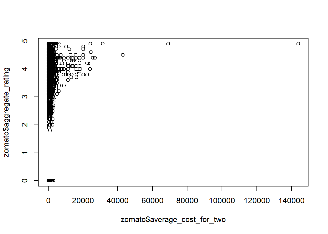
When we summary, maximum value of the order is 143927 and minimum value is 0. But order value varies between 300 to 700 most of the time. We need to check whether the Min and Max values are outlier or not and how many values are below 300 and more than 700. The value 300 is 1st Quartile and value 700 is third quartile. Let’s find out how many values are more than 3rd quartile 700:
nrow(zomato[zomato$average_cost_for_two>700,])
[1] 2380
The number of observations where value of average_cost_for_two is more than 700 are 2380 which is approx. 25% of the total observations in the dataset which is huge. We can discard the observations carrying 700+ value of average_cost_for_two. Let’s see the visualisation box plot for this:
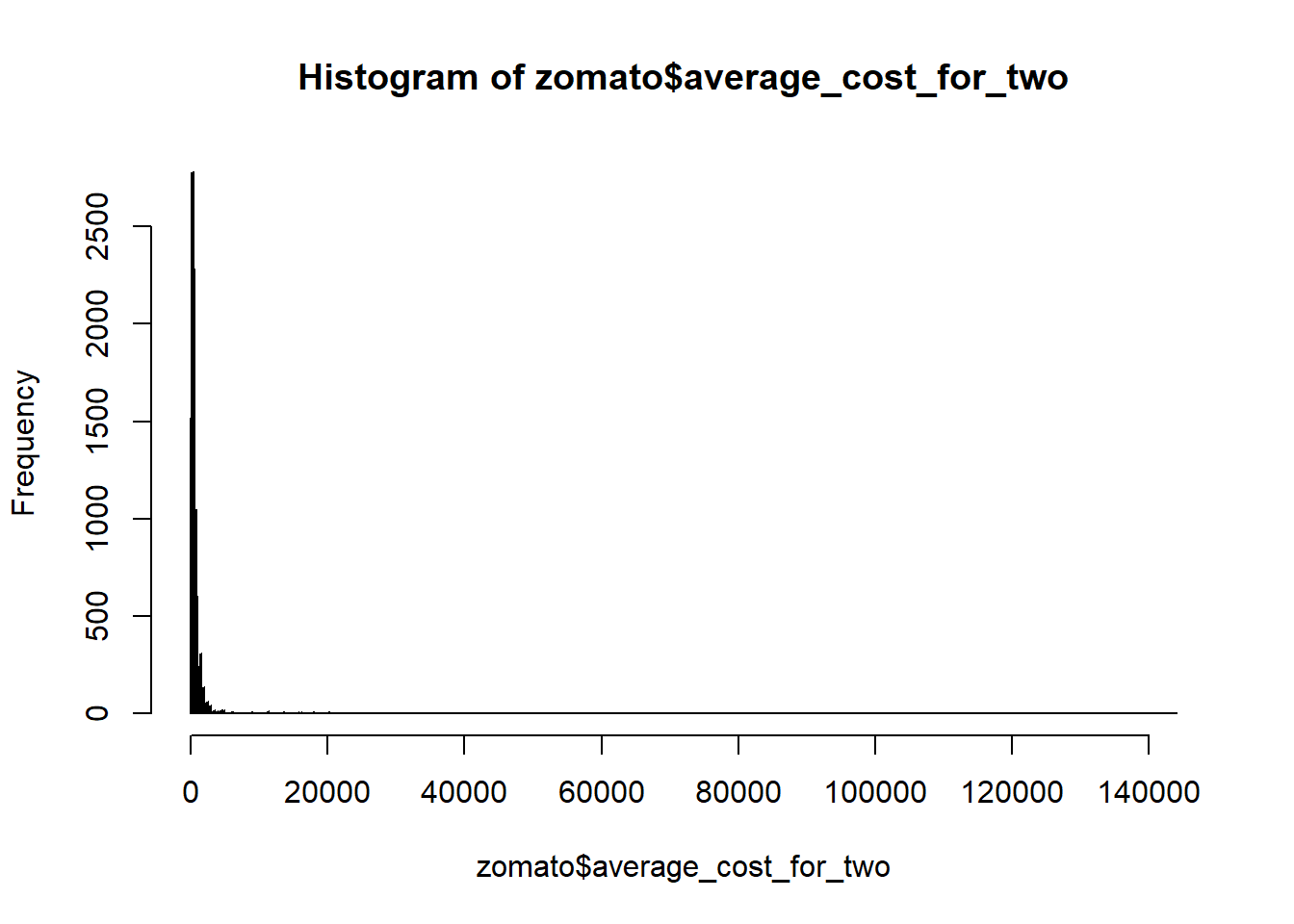
hist(zomato$average_cost_for_two, n=1000)
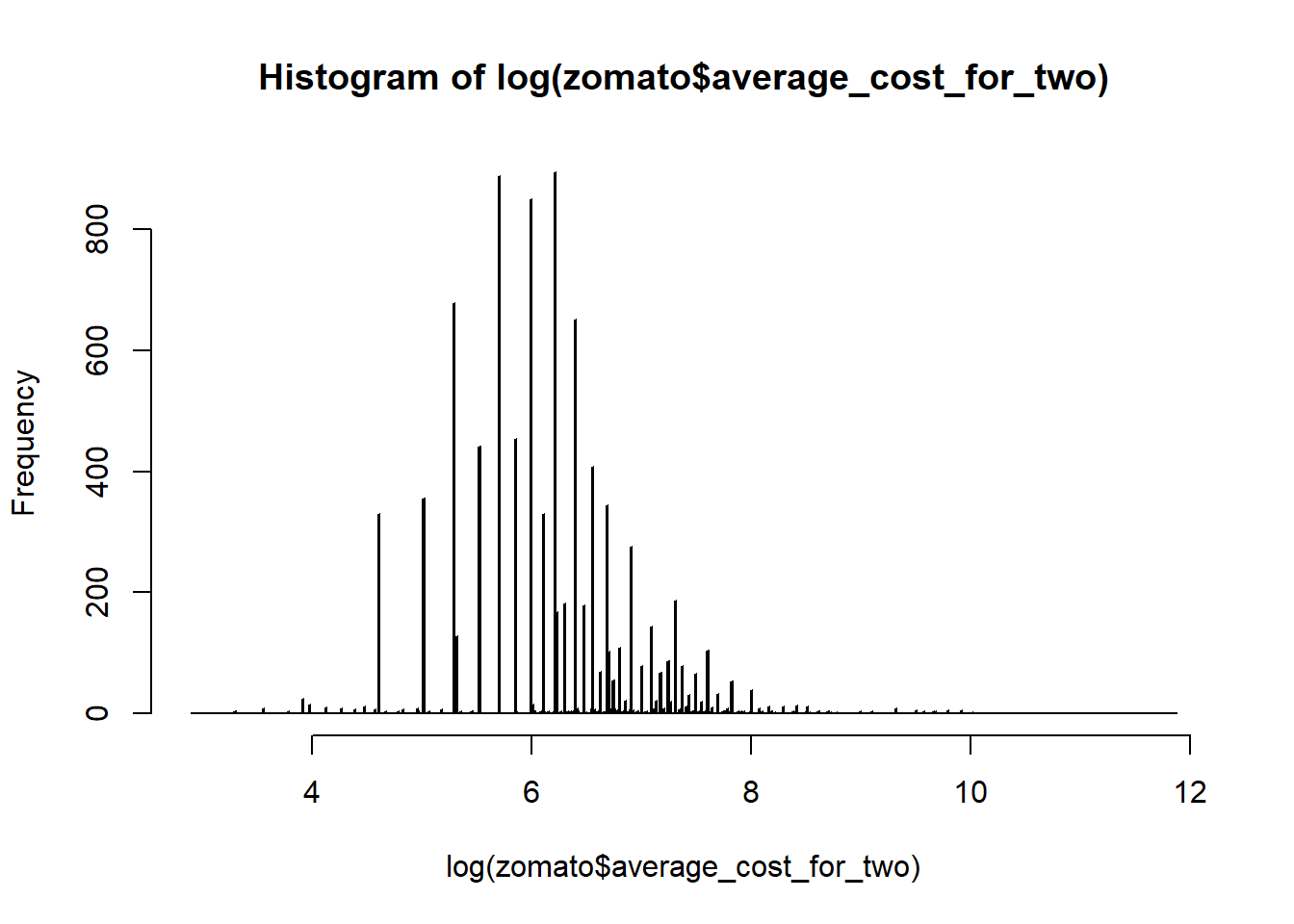
We can see that the density plot of the average cost is right skewed due to presence of outliers on the higher side. Let’s plot the log form of this and see what happens:
In the plot, we can see that the distribution of average_cost_for_two values is normally distributed. We will use the log value for further data analysis now. We add new variable log_avg_cost to the dataset:
We learnt one method of data transformation here i.e. log transformation to achieve normality in the data. Normality of data is an important factor in the data analysis. Many statistical theories, tests and models assume that the variable values should be normally distributed. To comply with that we transform the variable to get closer to the normal distribution.
Other type of transformations and their application criteria is as follows:
Data Transformation Type
Criteria to Apply
Sample Command in R
Log Transformation
Data is right-skewed; variance increases with mean
log(x) or log1p(x) (for zero values)
Square Root Transformation
Count data or moderately skewed data
sqrt(x)
Standardization (Z-score)
Variables on different scales; need mean 0, sd 1
scale(x)
Min-Max Normalization
Scale data to [0,1] for machine learning
(x - min(x)) / (max(x) - min(x))
Box-Cox Transformation
Data is positive and skewed; find best power transform
library(MASS); boxcox(lm(y ~ x))
Categorical Encoding
Convert factors for modeling
as.numeric(factor(x)) or model.matrix(~x-1)
Logit Transformation
Data is proportion/fraction in (0,1)
log(x / (1 - x))
Differencing
Time series with trends to make stationary
diff(x)
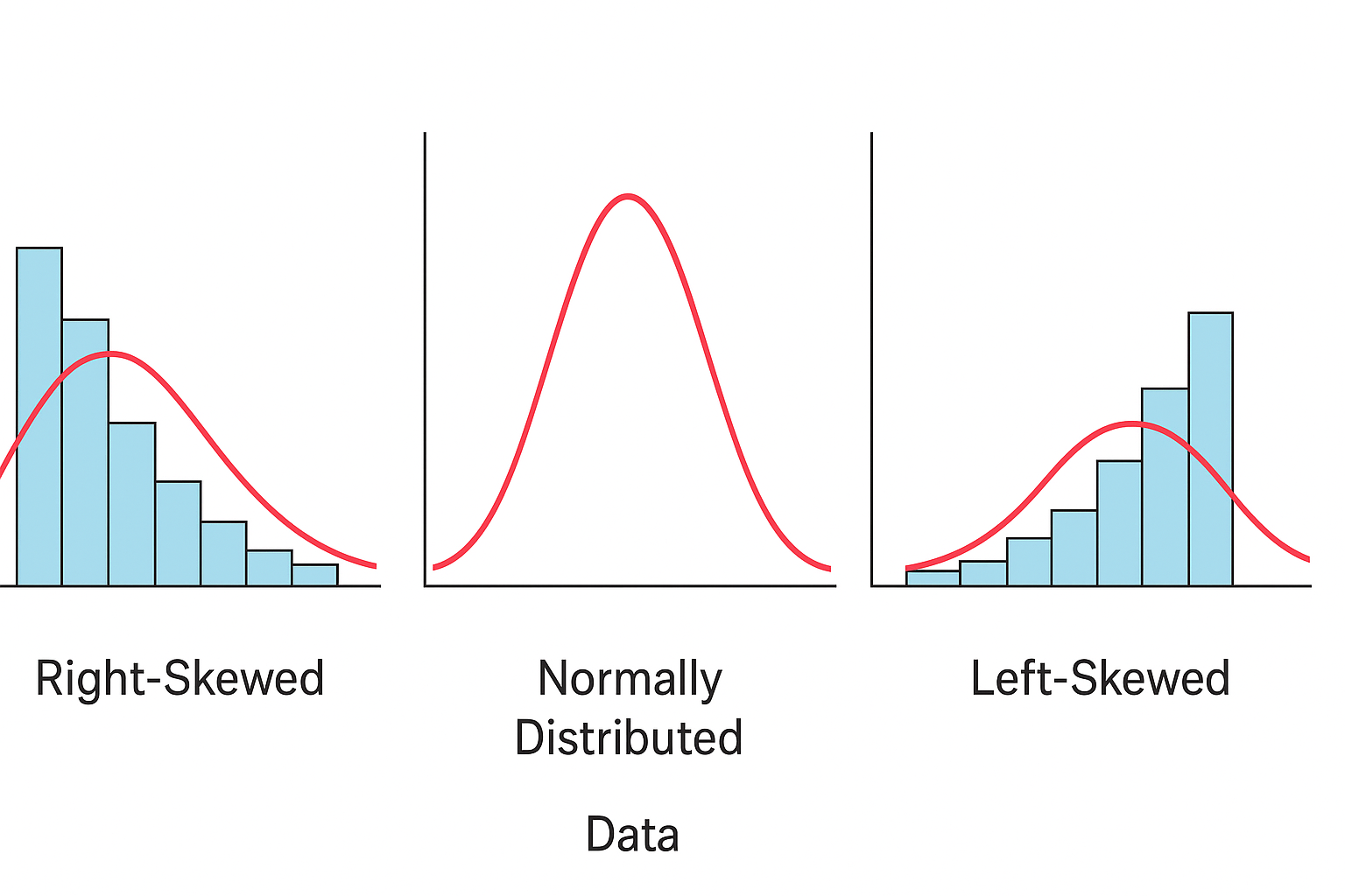
Purpose of transformation to achieve the normality in the data as per the middle figure shown here:
Variable price_range contains four repeating values - 1,2,3 and 4. Let’s change this variable from integer to factor variable:
zomato$price_range =as.factor(zomato$price_range)
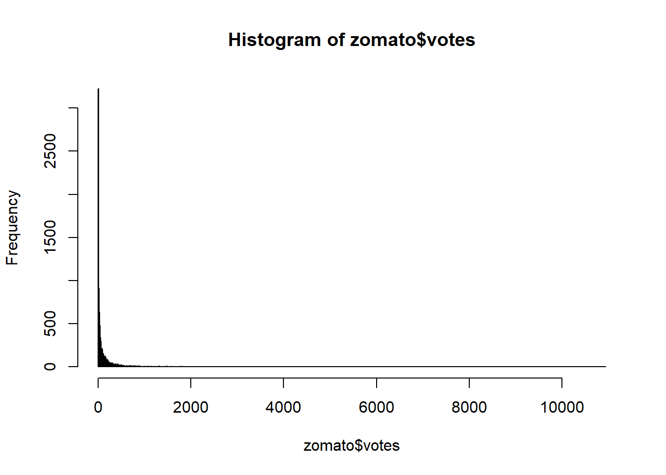
Let’s also see how values of votes are distributed:
hist(zomato$votes, n=1000)
We don’t transform votes variable in spite of the fact that the data is normally distributed because the votes are abolute values which we will use to rank different restaurants.
Data standardization is used when we have two different variables measured in different units needs to be compared. With standardization, variables are scaled on common scale, usually between 0 and 1.
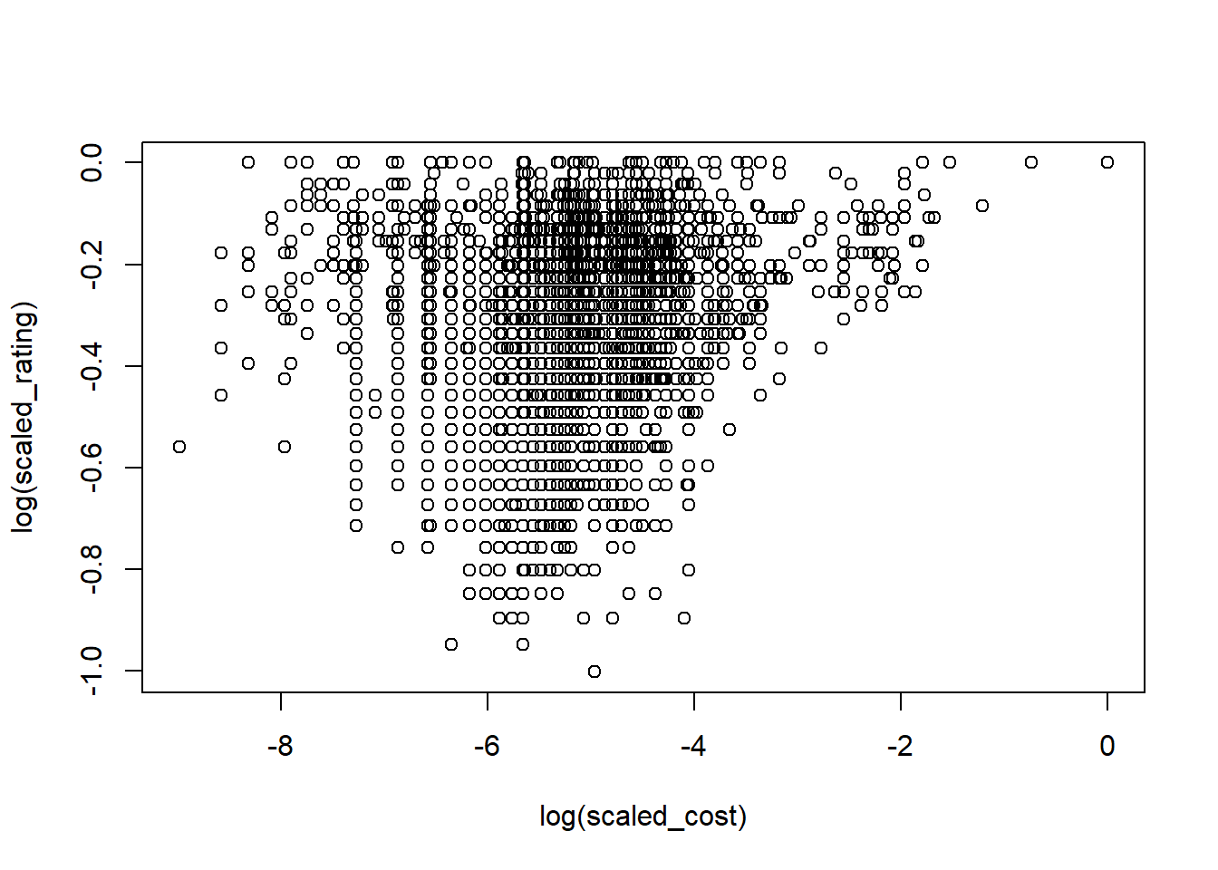
Now, we standardize the variables between 0 and 1 with function min_max_scale and then we log transform both variable and create a scatter plot:
min_max_scale <-function(data) {# Avoid division by zero if all values are the sameif (max(data) ==min(data)) {return(rep(0, length(data))) }return((data -min(data)) / (max(data) -min(data)))}scaled_cost =min_max_scale(zomato$average_cost_for_two)scaled_rating =min_max_scale(zomato$aggregate_rating)plot(log(scaled_cost), log(scaled_rating))
This plot gives better visualization of the interaction between two variables then the previous one.
 In this window, give name to your directory in the box “Directory Name” and set the directory path with browse option. Now, click the
 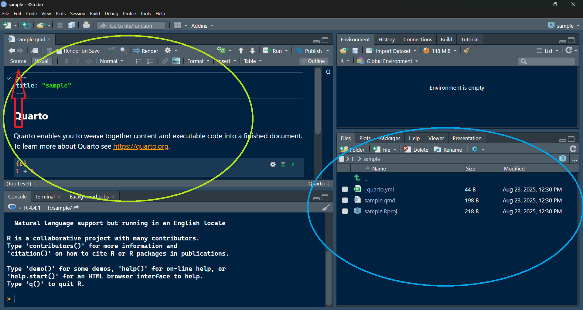 In the output pane (in blue circle), you can see that there are three files are created-